Paths

Background

This vignette develops the paths. The topics include introducing simplex noise, the functions that move the anchor points, and investigating direction correlations. Reading the other vignettes first will be helpful.

Simplex Noise

To create the paths the points follow, this package uses noise-generating functions from the ambient package. These functions make a smooth terrain the points can flow through. Saving each step and then graphing them draws the paths. There are many functions, each with several parameters, and they can be combined for a ton of options. However, this package only uses one type of simplex noise. We’ll need to generate some points to see it in action.

library(tidyverse)
library(ambient)
library(purrr)

points <- expand_grid(
  x = seq(1, ceiling(sqrt(750))) - (ceiling(sqrt(750)) / 2) - .5,
  y = seq(1, ceiling(sqrt(750))) - (ceiling(sqrt(750)) / 2) - .5
) %>%
  mutate(
    x = x * 5, # get to the right scale
    y = y * 5,
    id = dplyr::row_number()
  )

ggplot(
  data = points,
  aes(x, y)
) +
  geom_point(size = .5) +
  coord_equal()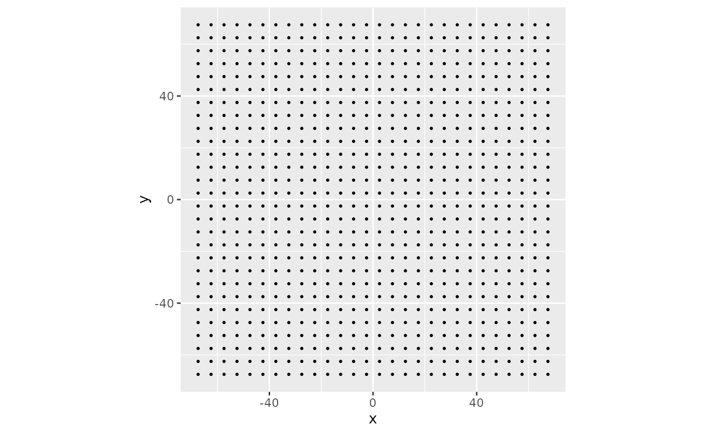

Points Setup

In the code for this grid, the x and y values are scaled by 5. This scale will set up the amount of movement in the paths I’m trying to find. The paths will be too similar if the points are too close together. If they are too far apart, they will be too different. This scale and almost every number will depend on what you are attempting. There’s not really a mathematical optimization here. It’s just playing around with parameters until you get something you like.

The following line actually generates the noise. It takes in the x and y values as the locations. The frequency parameter sets how much movement happens, while the seed parameter ensures the exact same results can occur. This feature will be important in a second.

points <- points %>%
  mutate(noise = gen_simplex(x,
    y,
    frequency = .01,
    seed = 1
  ))

ggplot(
  data = points,
  aes(noise)
) +
  geom_histogram(bins = 25)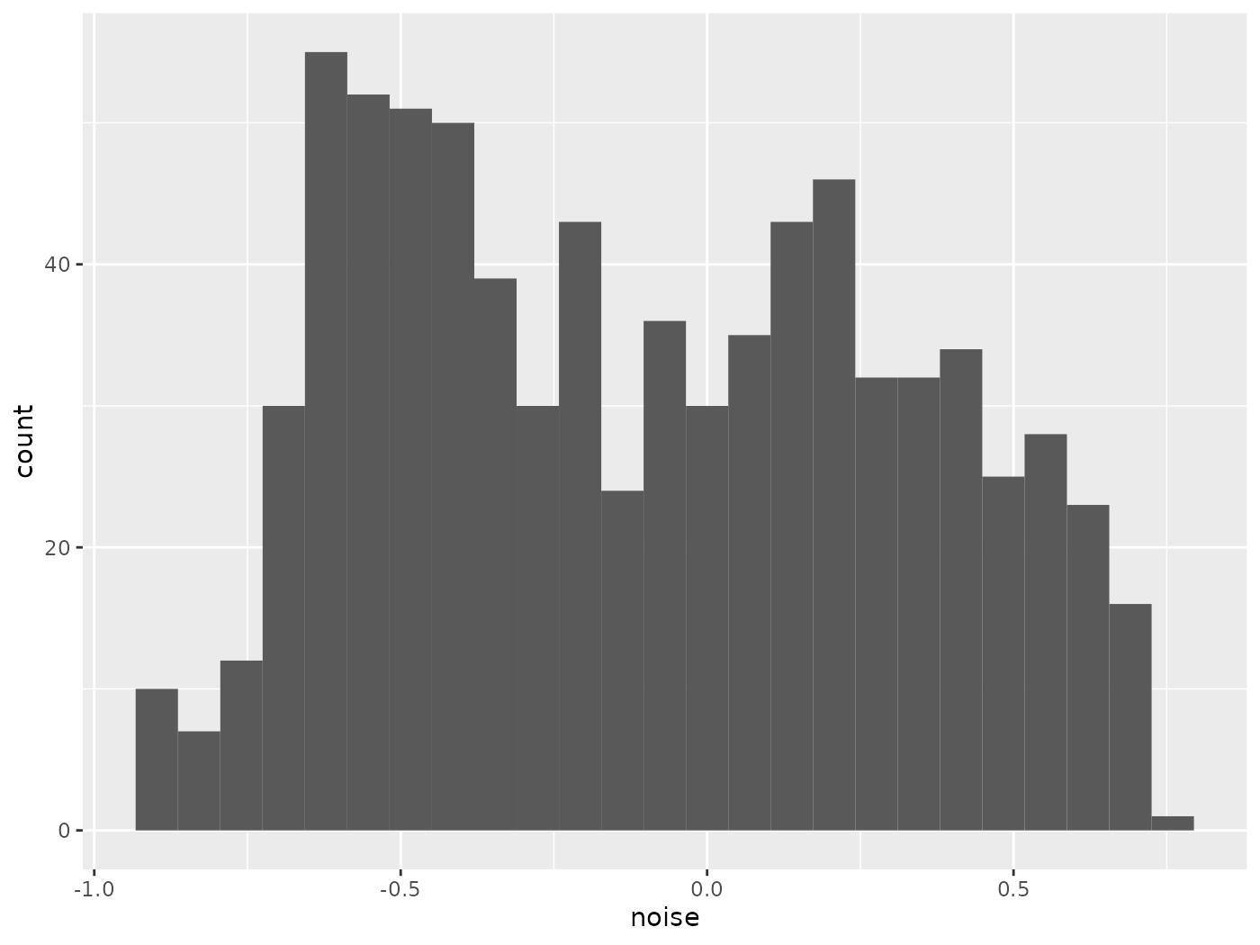

Simplex Histogram

ggplot(
  data = points,
  aes(x, y, fill = noise)
) +
  geom_tile() +
  coord_equal()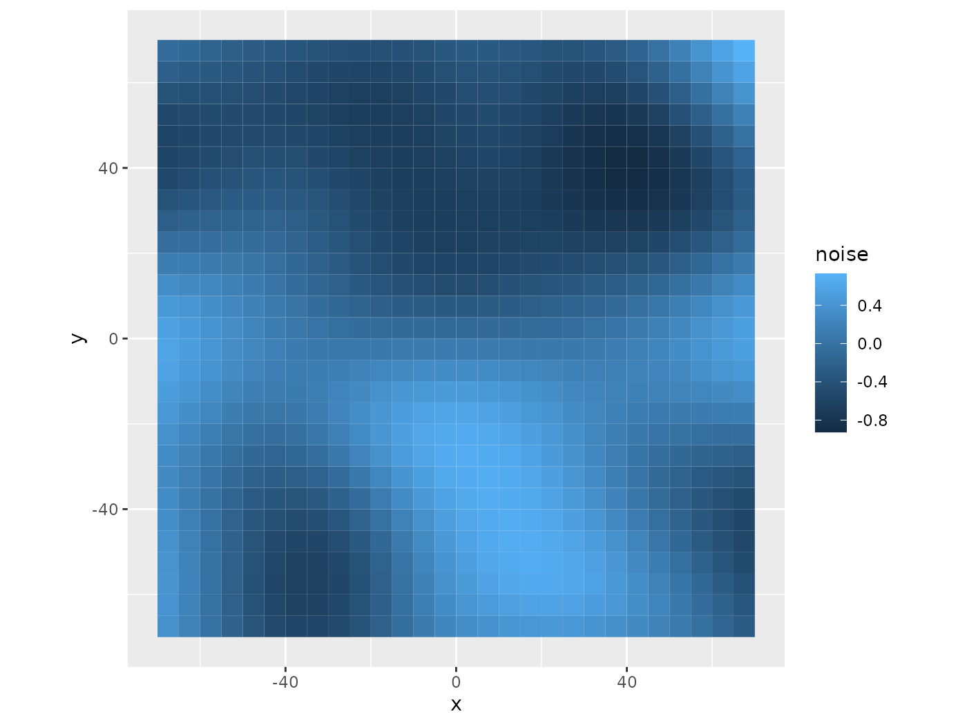

Simplex Map

The results show that the noise values are between -1 and 1, tend to slope off at the ends, but are also multimodal. These attributes typically hold for this set of points and this noise-generating function, even with a different seed, but won’t always happen with other options. The map on the right shows the terrain. Using only this noise to create paths, they’ll move from higher values to lower ones. However, this package will use a different technique.

To understand the importance of the seed parameter, we can move the points with the same seed and a different one to see what happens. Moving the points up and over with the same seed generates almost the same map. It’s the same terrain, but the view has shifted with the points. The same movement with a different seed yields an entirely different map. This new map won’t be usable if the paths need to follow the same hills and valleys. Therefore, the code requires the seed parameter to generate the same noise values for the points to use as they move. This feature is very nice when the points don’t move along a grid and can end up anywhere.

points_move <- points %>%
  mutate(
    x = x + 1,
    y = y + 1
  ) %>%
  mutate(noise = gen_simplex(x,
    y,
    frequency = .01,
    seed = 1
  ))

ggplot(
  data = points_move,
  aes(x, y, fill = noise)
) +
  geom_tile() +
  coord_equal()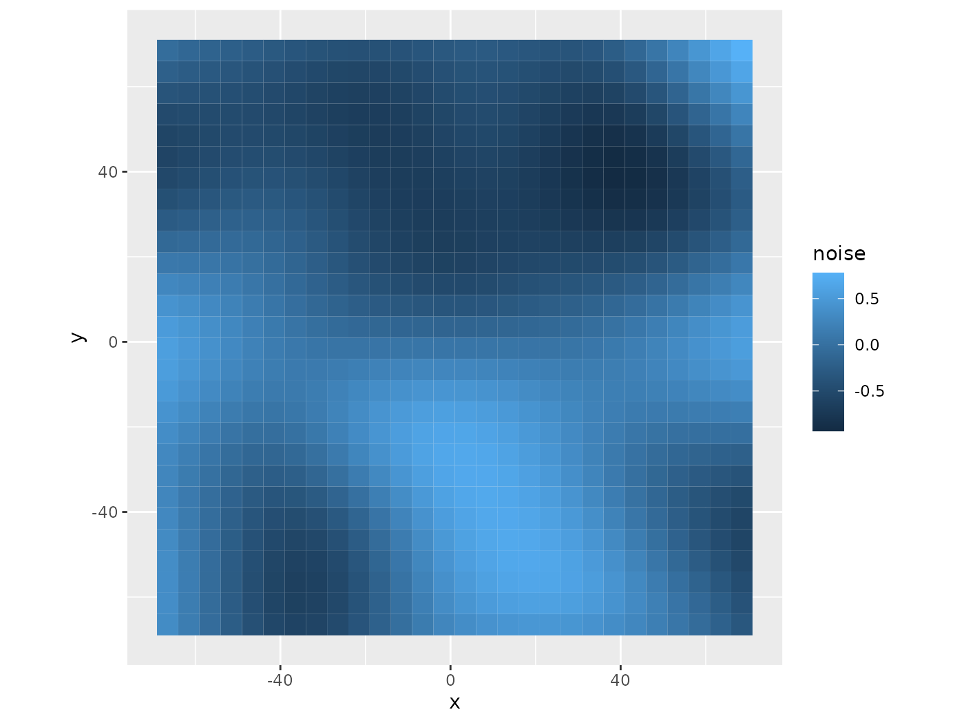

Simplex Map Movement Same Seed

points_move <- points %>%
  mutate(
    x = x + 1,
    y = y + 1
  ) %>%
  mutate(noise = gen_simplex(x,
    y,
    frequency = .01,
    seed = 2
  ))

ggplot(
  data = points_move,
  aes(x, y, fill = noise)
) +
  geom_tile() +
  coord_equal()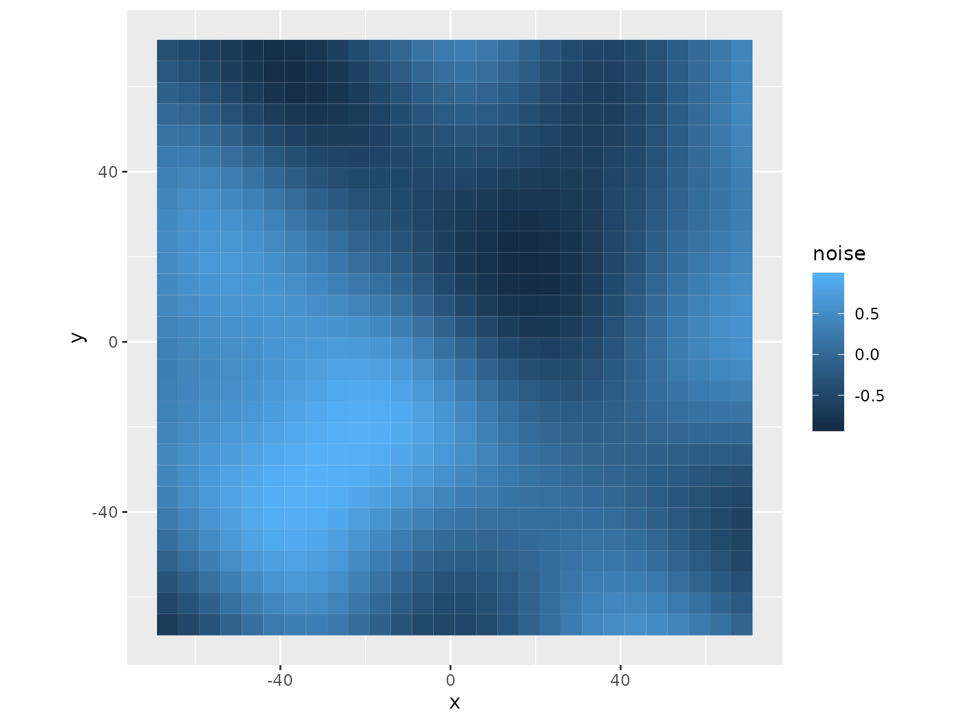

Simplex Map Movement Different Seed

While it would be great to use this noise as terrain, we really need the slope and not elevation to get movement. The gradient_noise function in ambient is probably the best choice for this, but I decided to see other options.

It’s possible to take the noise and wrap it to be an angle. However, each run of the noise function can have different bounds. So, we struggle to set up the values as angles without any gaps or large directions.

ggplot(
  data = points,
  aes(noise)
) +
  geom_histogram(bins = 25) +
  coord_polar()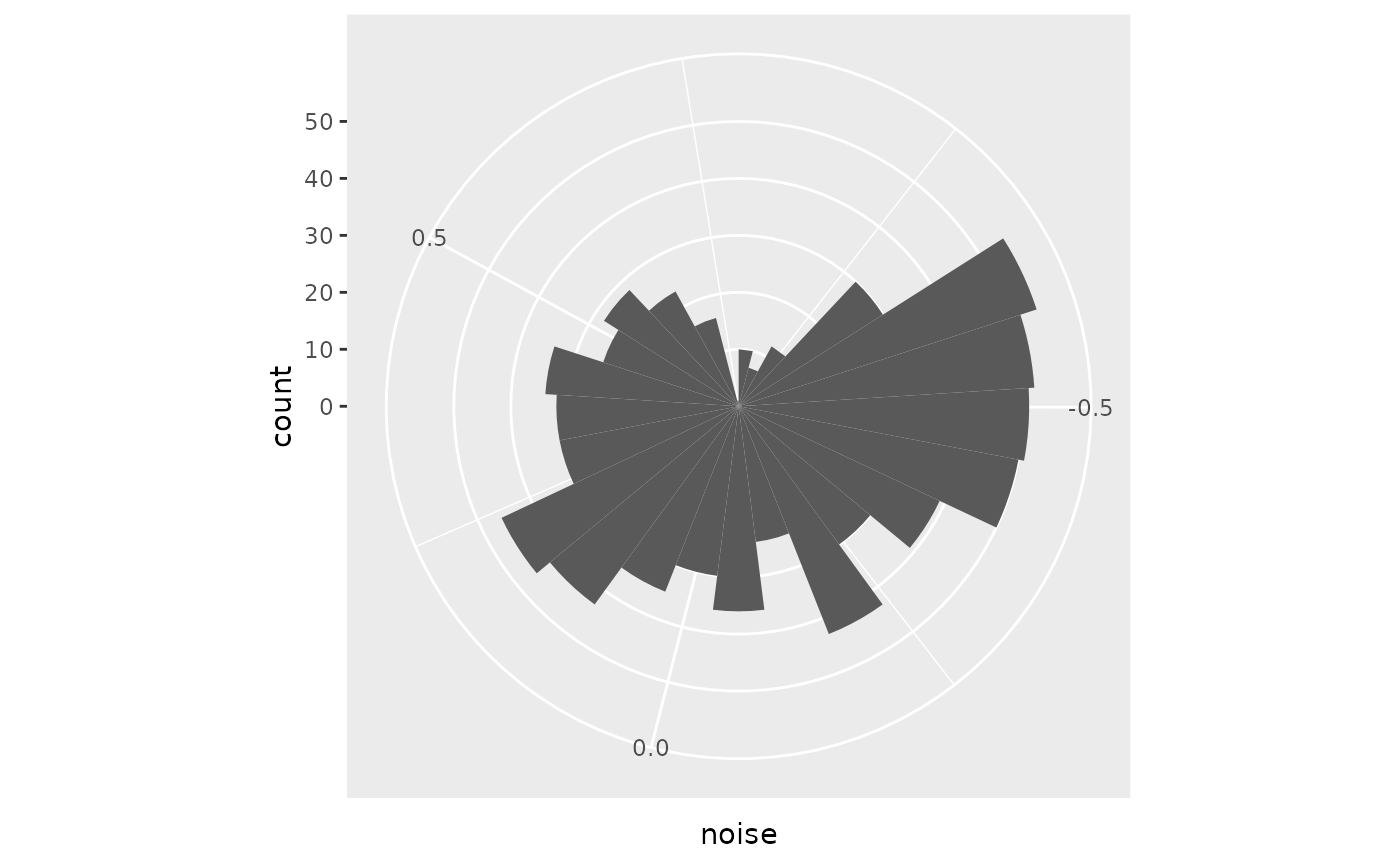

Angle Attempt

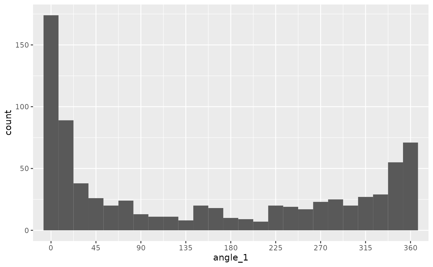
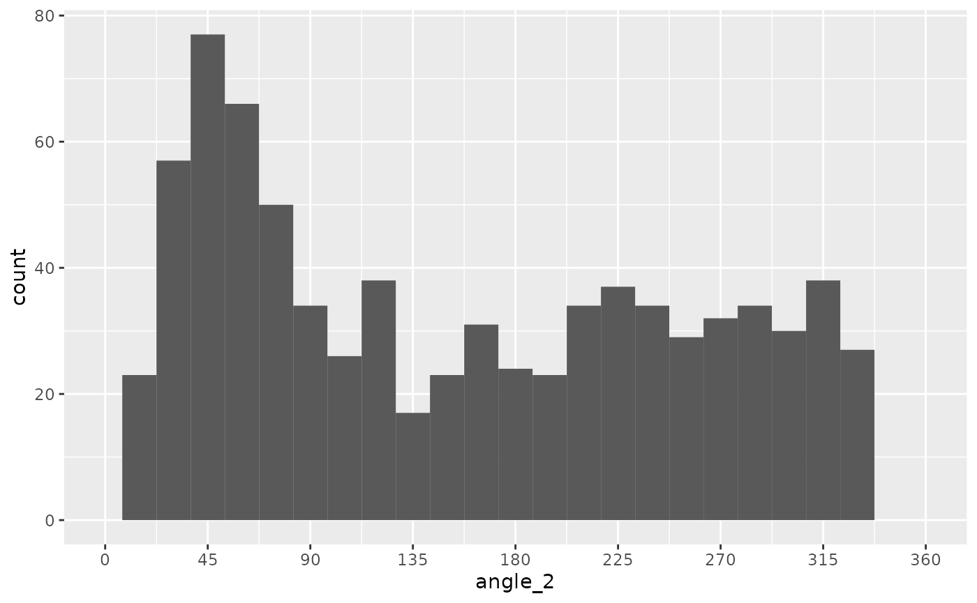
The following code section tries different techniques to transform the noise values into angles. Unfortunately, there are problems with gaps or significant modes on these values. I didn’t like that for this project, but these could be desirable attributes for something else.

points <- points %>%
  mutate(
    angle_1 = (pnorm(noise, sd = .25) * 360),
    angle_2 = (pnorm(noise, sd = .5) * 360),
    angle_3 = (1 / (1 + exp(-noise / .25)) * 360)
  )

ggplot(
  data = points,
  aes(angle_1)
) +
  geom_histogram(bins = 25) +
  scale_x_continuous(
    limits = c(0, 360),
    oob = scales::oob_keep,
    breaks = seq(0, 360, 45)
  )

pnorm(sd = .25)

ggplot(
  data = points,
  aes(angle_2)
) +
  geom_histogram(bins = 25) +
  scale_x_continuous(
    limits = c(0, 360),
    oob = scales::oob_keep,
    breaks = seq(0, 360, 45)
  )

pnorm(sd = .25)

ggplot(
  data = points,
  aes(angle_3)
) +
  geom_histogram(bins = 25) +
  scale_x_continuous(
    limits = c(0, 360),
    oob = scales::oob_keep,
    breaks = seq(0, 360, 45)
  )

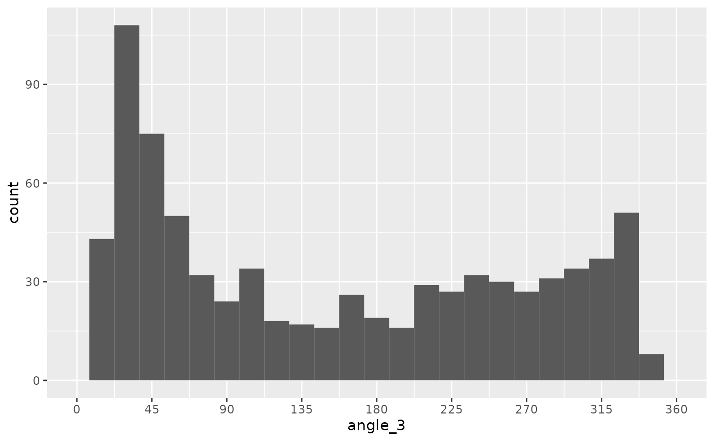
logistic

ggplot(
  data = points,
  aes(angle_1)
) +
  geom_histogram(bins = 25) +
  scale_x_continuous(
    limits = c(0, 360),
    oob = scales::oob_keep,
    breaks = seq(0, 360, 45)
  ) +
  coord_polar(
    direction = -1,
    start = 270 * pi / 180
  )

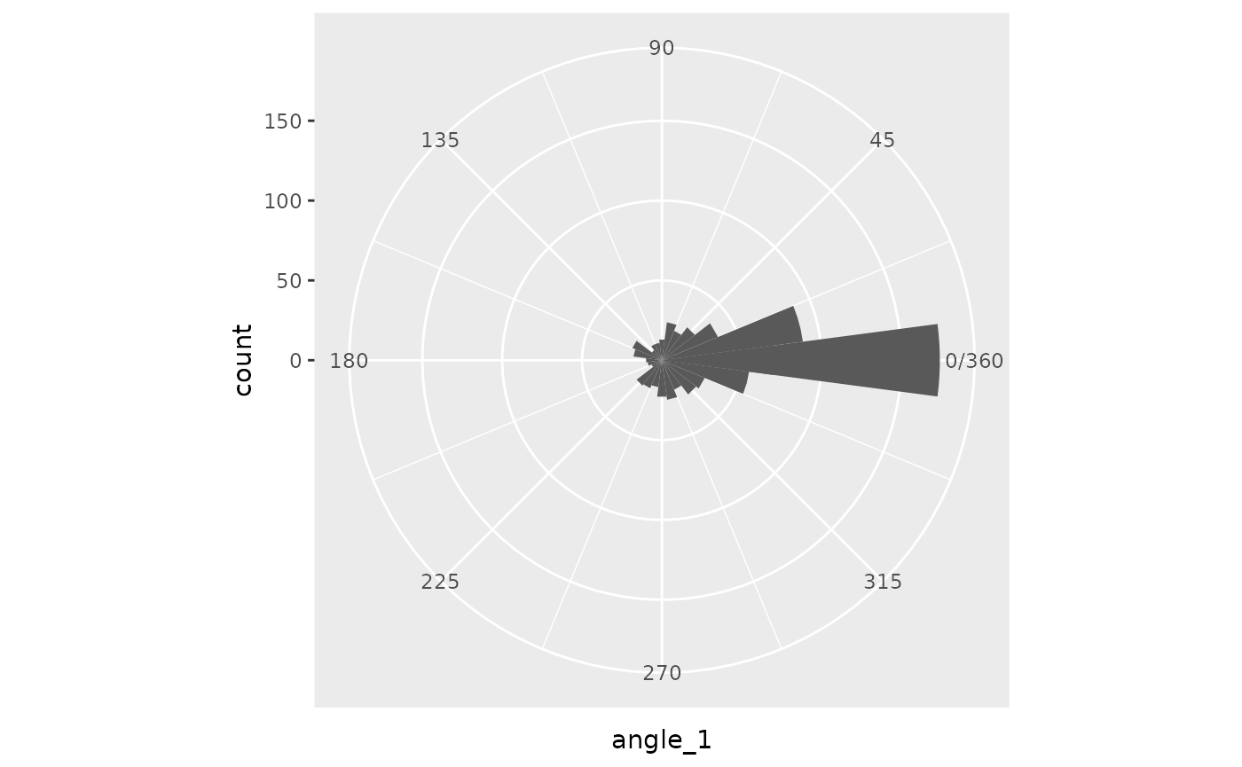
pnorm(sd = .25)

ggplot(
  data = points,
  aes(angle_2)
) +
  geom_histogram(bins = 25) +
  scale_x_continuous(
    limits = c(0, 360),
    oob = scales::oob_keep,
    breaks = seq(0, 360, 45)
  ) +
  coord_polar(
    direction = -1,
    start = 270 * pi / 180
  )

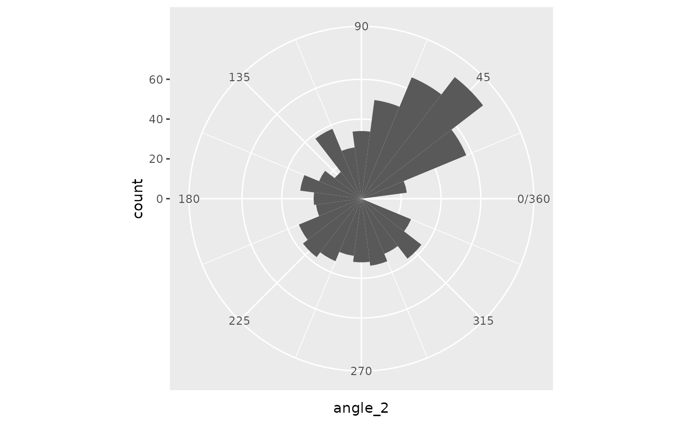
pnorm(sd = .25)

ggplot(
  data = points,
  aes(angle_3)
) +
  geom_histogram(bins = 25) +
  scale_x_continuous(
    limits = c(0, 360),
    oob = scales::oob_keep,
    breaks = seq(0, 360, 45)
  ) +
  coord_polar(
    direction = -1,
    start = 270 * pi / 180
  )

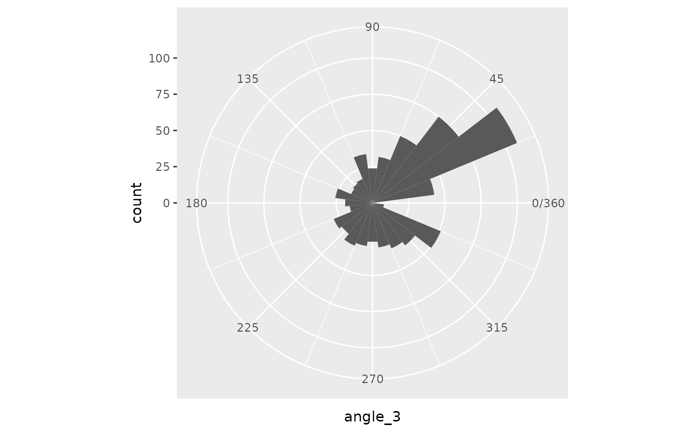
logistic

Using simplex noise is flawed in that it only provides one dimension, and we really need two, one for x movement and one for y. So, let’s just use two simplex noises, one for each direction. (Agina, there are options to resolve this if you want one function, like curl noise.)

points <- expand_grid(
  x = seq(1, ceiling(sqrt(750))) - (ceiling(sqrt(750)) / 2) - .5,
  y = seq(1, ceiling(sqrt(750))) - (ceiling(sqrt(750)) / 2) - .5
) %>%
  mutate(
    x = x * 5, # get to the right scale
    y = y * 5,
    id = dplyr::row_number()
  )

points <- points %>%
  mutate(
    x_direction = gen_simplex(x,
      y,
      frequency = .01,
      seed = 1
    ),
    y_direction = gen_simplex(x,
      y,
      frequency = .01,
      seed = 2
    )
  )

The following graphs show the movement in the x-direction and y-direction. They are different locations for the hills and valleys, but the ranges are similar. Because each simplex noise function has the same parameters, except seed, the results are similar in smoothness.

ggplot(
  data = points,
  aes(x, y, fill = x_direction)
) +
  geom_tile() +
  scale_fill_continuous(limits = c(-1, 1)) +
  coord_equal()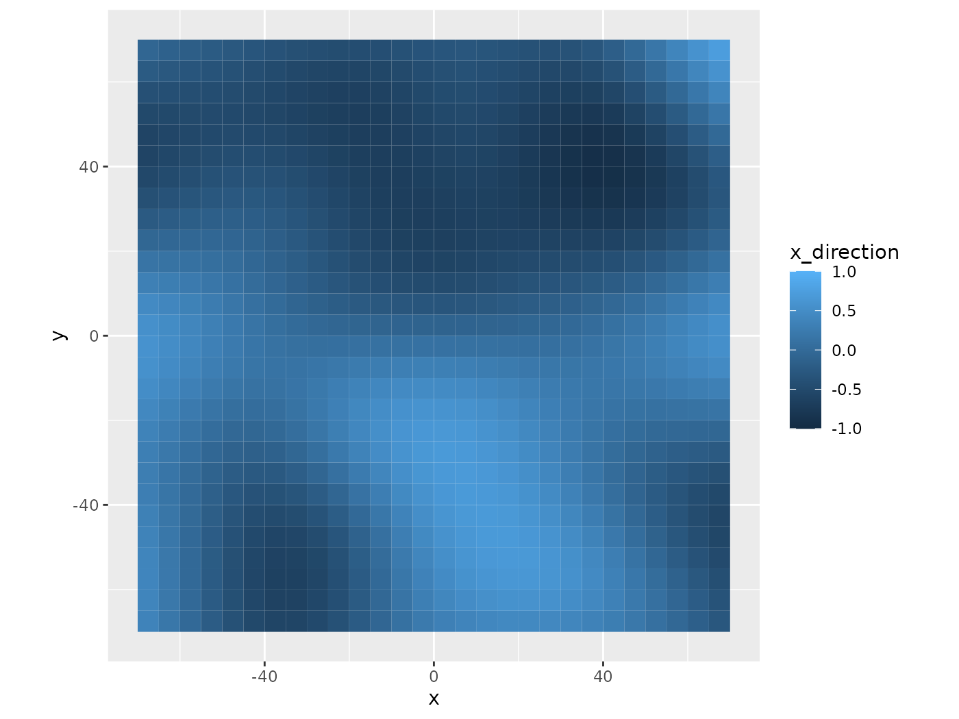

X Movement

ggplot(
  data = points,
  aes(x, y, fill = y_direction)
) +
  geom_tile() +
  scale_fill_continuous(limits = c(-1, 1)) +
  coord_equal()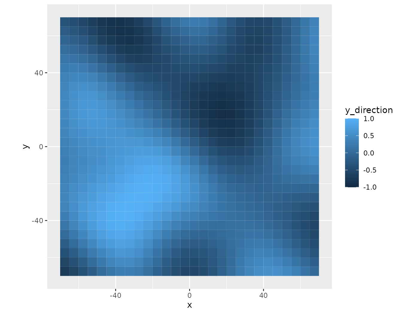

Y Movement

We can standardize the movements to have each step be the same distance. This is useful because we set up the points to have their own distances for how far the paths should go. Then, the standardized movements render the angle.

points <- points %>%
  mutate(vector_length = sqrt(x_direction^2 +
    y_direction^2)) %>%
  mutate(
    x_direction = x_direction / vector_length,
    y_direction = y_direction / vector_length
  ) %>%
  select(-vector_length) %>%
  mutate(angle = (atan2(y_direction, x_direction) * 180 / pi) %% 360)

The following graphs of the standardized movements show how each directions’ values affect the other. These are a blend of the two previous graphs while remaining different. There is also a larger range of movement and sharper changes in direction.

ggplot(
  data = points,
  aes(x, y, fill = x_direction)
) +
  geom_tile() +
  scale_fill_continuous(limits = c(-1, 1)) +
  coord_equal()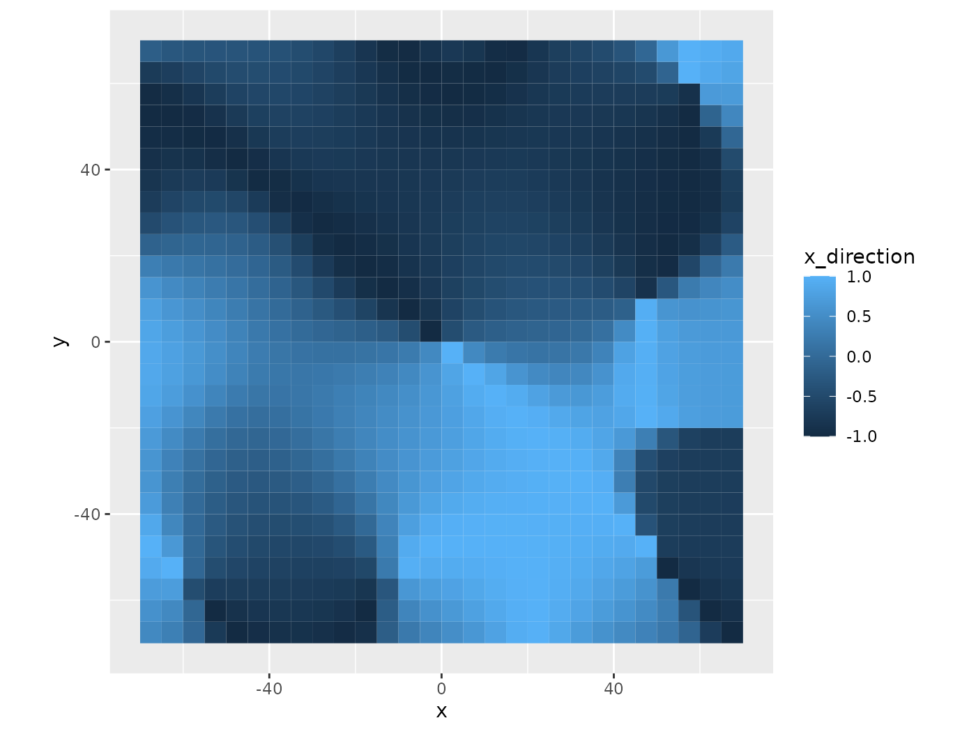

X Movement Standardized

ggplot(
  data = points,
  aes(x, y, fill = y_direction)
) +
  geom_tile() +
  scale_fill_continuous(limits = c(-1, 1)) +
  coord_equal()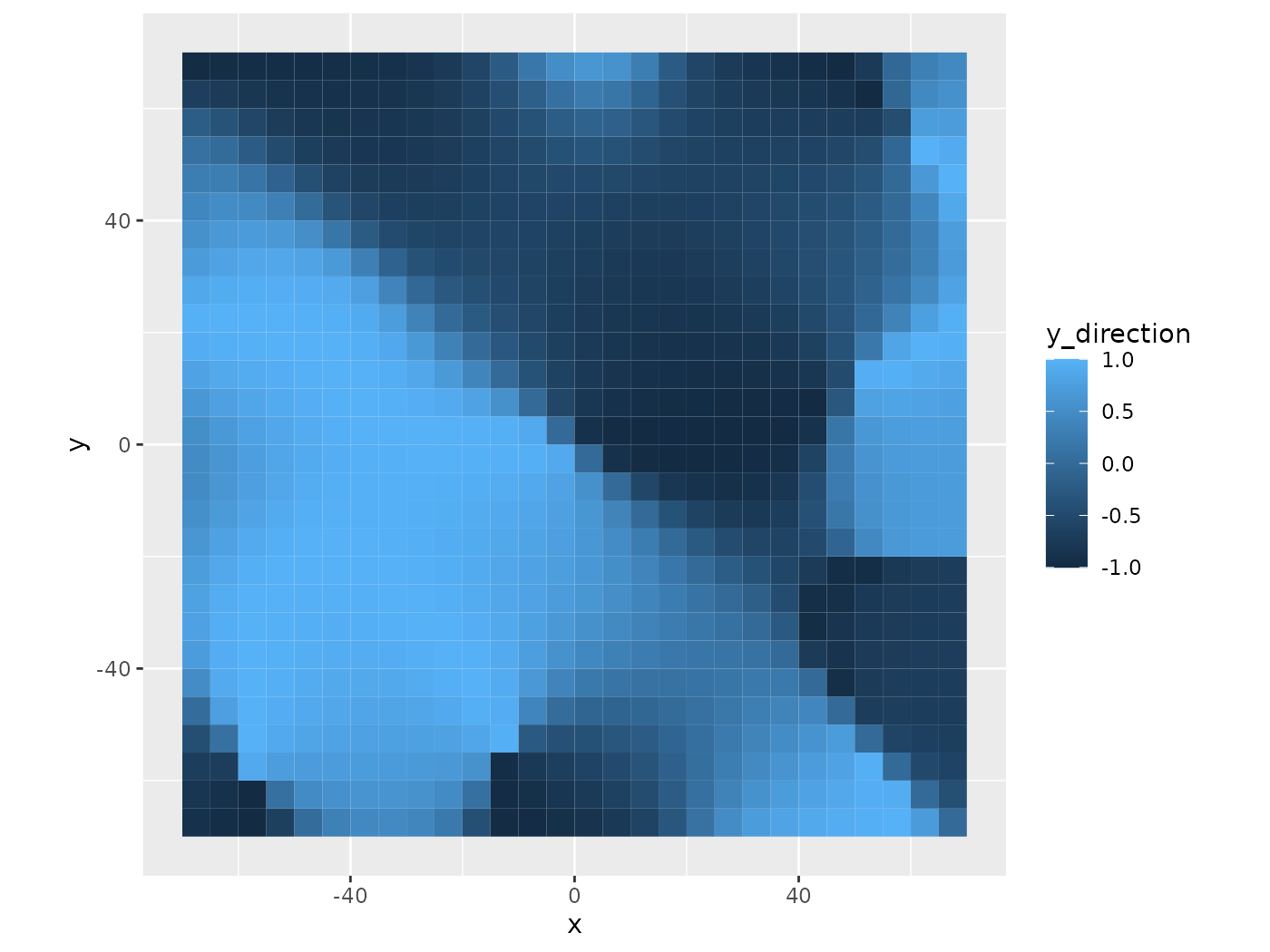

Y Movement Standardized

Here we have the starting directions from all this work. There are primarily smooth transitions from one arrow to its neighbor. There are areas with little change and areas with a lot. Also, notice that the block from (-40, 0) to (0, 40) is a lot smoother than the block from (-20, -20) to (20, 20). For some reason, (0, 0) always has a lot of action. I suspect it has something to do with the simplex noise generation process at the origin.

ggplot(
  data = points,
  aes(x, y, 
      xend = x + x_direction,
      yend = y + y_direction,
      color = angle)
) +
  geom_segment(arrow = arrow(length = unit(0.033, "inches"))) +
  scale_colour_gradient2(
    low = "darkblue",
    mid = "lightblue",
    high = "darkblue",
    midpoint = 180,
    breaks = seq(0, 360, 90)
  ) +
  coord_equal()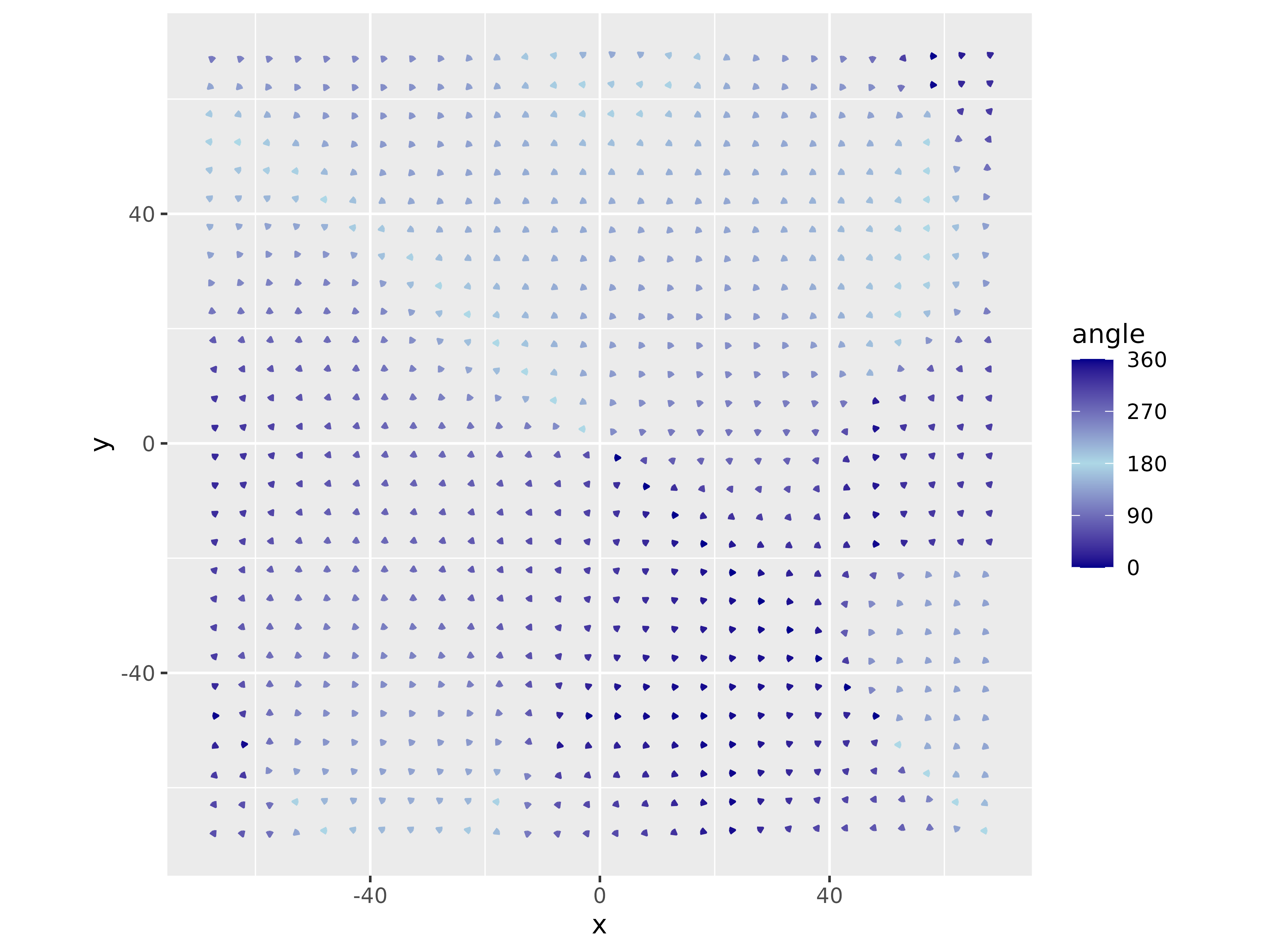 

Angle Map

Finally, we see the overall angle distribution. The histogram shows large values around 225, but smaller than the previous graph with one mode. There is also a lack of values at 270, but it’s not a complete gap to 0.

ggplot(
  data = points,
  aes(angle)
) +
  geom_histogram(bins = 25) +
  scale_x_continuous(
    limits = c(0, 360),
    oob = scales::oob_keep,
    breaks = seq(0, 360, 45)
  ) +
  coord_polar(
    direction = -1,
    start = 270 * pi / 180
  )

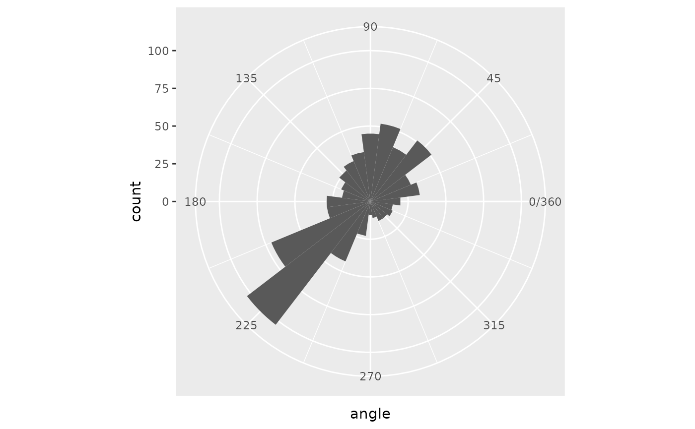
Angle Histogram

Now that we have a mechanism to get the direction at any spot, we can use it to create paths.

Moving Points

Danielle Navarro’s “Art, jasmines, and the water colours” post heavily influenced this section. I highly recommend reading it to understand this code better and see another way to use flow fields for generative art.

We’ll create two helper functions: one to get the directions and one to add the movement to points. get_vectors uses the points’ current location and a set of seeds to return the direction the points should move. move_points adds the distances to the points and updates the time. Following the points along all time values will display the paths. These two functions can be written into only one if we just need the paths. Setting up the colors uses get_vectors and not move_points, so they’ll stay separated for this project.

get_vectors <- function(points, seeds) {
  vectors <- points %>%
    mutate(
      x_direction = gen_simplex(x,
        y,
        frequency = .01,
        seed = seeds[1]
      ),
      y_direction = gen_simplex(x,
        y,
        frequency = .01,
        seed = seeds[2]
      )
    ) %>%
    mutate(vector_length = sqrt(x_direction^2 +
      y_direction^2)) %>%
    mutate(
      x_direction = x_direction / vector_length,
      y_direction = y_direction / vector_length
    ) %>%
    select(-vector_length)
}

move_points <- function(points, seeds) {
  points <- points %>%
    get_vectors(seeds) %>%
    mutate(
      x = x + x_direction * .5,
      y = y + y_direction * .5,
      time = time + 1
    )
  return(points)
}

We’ll now create the primary function, get_paths, that uses the two other functions. This function uses accumulate from the purrr package. We’ll start with our set of points, apply move_points 100 times and pass the seeds to get the same noise values. This action returns a data frame for each step, which we’ll bind together. Lastly, we’ll get the next step along the paths and filter out points that don’t have the next step or need to be shortened based on their percentage value. Points will not have a next step at the end or if they move to a completely flat area and get stopped. (percentage comes from setting up the points, see their vignette.)

get_paths <- function(points, seeds) {
  paths <- accumulate(
    .x = rep(list(seeds), 100), # up to 100 for max percentage
    .f = move_points,
    .init = points
  )
  paths <- bind_rows(paths)
  paths <- paths %>%
    group_by(id) %>%
    mutate(
      xend = lead(x),
      yend = lead(y)
    ) %>%
    filter(!is.na(xend)) %>%
    filter(time <= percentage)
}

Now we can reset our points, get some seeds, and try out this function. First, we’ll set all the percentage values to 50. All the paths will be the same length for this example. In the output, we can see each step a point takes by looking at x, y, xend, and yend

points <- expand_grid(
  x = seq(1, ceiling(sqrt(750))) - (ceiling(sqrt(750)) / 2) - .5,
  y = seq(1, ceiling(sqrt(750))) - (ceiling(sqrt(750)) / 2) - .5
) %>%
  mutate(
    x = x * 5,
    y = y * 5,
    id = dplyr::row_number()
  )

set.seed(10000)
seeds <- sample(1:10000, 3)

points <- get_vectors(points, seeds) %>%
  mutate(
    time = 0,
    percentage = 50
  )

paths <- get_paths(points, seeds)

paths <- paths %>%
  arrange(id, time)

head(paths)
#> # A tibble: 6 × 9
#> # Groups:   id [1]
#>       x     y    id x_direction y_direction  time percentage  xend  yend
#>   <dbl> <dbl> <int>       <dbl>       <dbl> <dbl>      <dbl> <dbl> <dbl>
#> 1 -67.5 -67.5     1       0.447      -0.894     0         50 -67.3 -67.9
#> 2 -67.3 -67.9     1       0.447      -0.894     1         50 -67.1 -68.4
#> 3 -67.1 -68.4     1       0.435      -0.900     2         50 -66.8 -68.9
#> 4 -66.8 -68.9     1       0.423      -0.906     3         50 -66.6 -69.3
#> 5 -66.6 -69.3     1       0.411      -0.912     4         50 -66.4 -69.8
#> 6 -66.4 -69.8     1       0.399      -0.917     5         50 -66.2 -70.2

At the end of this section, we can finally see the paths. The square anchor points are still visible, but there is a lot of variability in where the points end and how they get there.

axes_limits <- max(c(abs(c(
  paths$x,
  paths$y,
  paths$xend,
  paths$yend
))))

ggplot(
  data = paths,
  aes(
    x = x,
    y = y,
    xend = xend,
    yend = yend
  )
) +
  geom_segment() +
  coord_equal()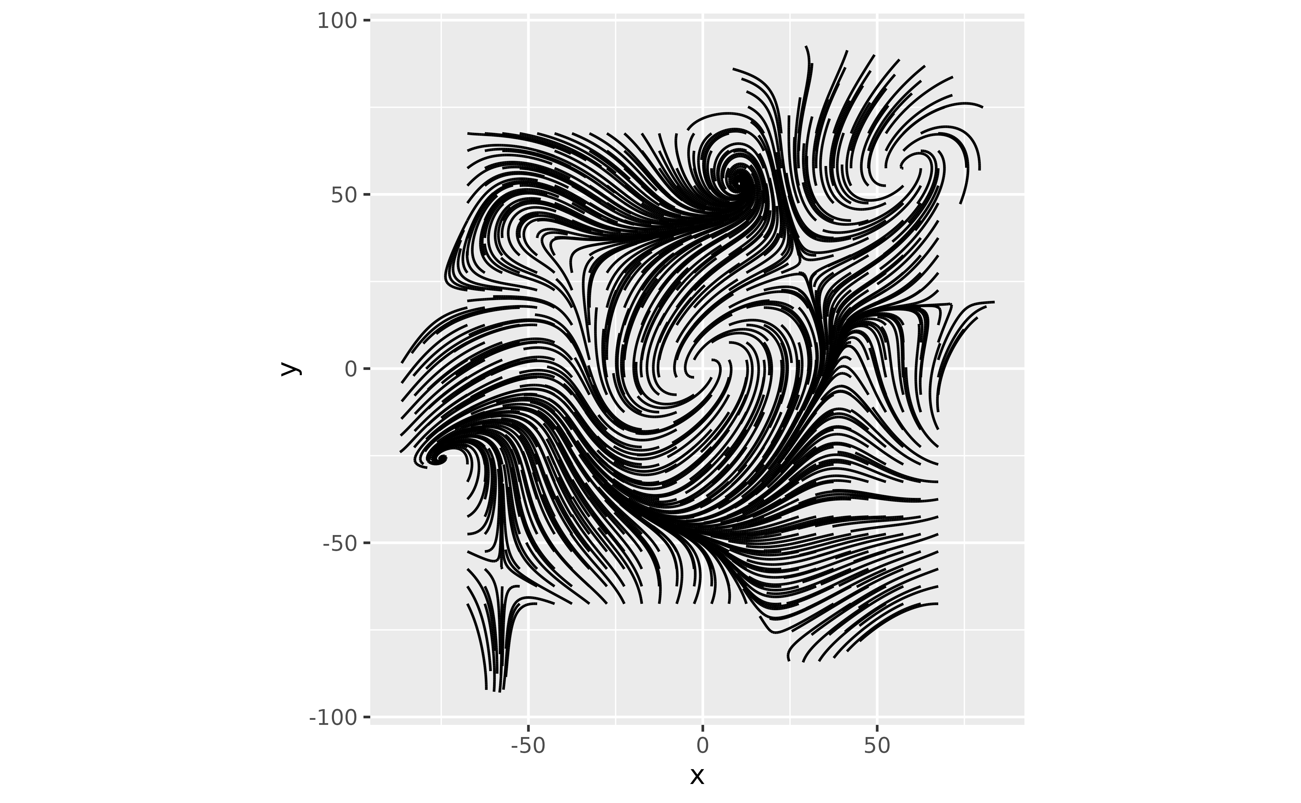

Paths Example

Common directions

We can look at all the steps taken to see any patterns. In this example, some angles are more common.

paths_direcion <- paths %>%
  ungroup() %>%
  mutate(angle = (atan2(y_direction, x_direction) * 180 / pi) %% 360) %>%
  mutate(angle = cut_interval(angle, n = 20, labels = FALSE) * (36 / 2) - (36 / 4)) %>%
  group_by(angle) %>%
  summarise(count = n())

ggplot(
  data = paths_direcion,
  aes(x = angle, y = count)
) +
  geom_bar(
    stat = "identity",
    width = 36 / 2
  ) +
  scale_x_continuous(
    limits = c(0, 360),
    breaks = seq(0, 360, 45)
  ) +
  coord_polar(
    direction = -1,
    start = 270 * pi / 180
  )

Paths Example

Let’s set up 100 attempts at the previous code and then aggregate them.

paths_direcion_score <- data.frame(
  run_id = integer(),
  angle = numeric(),
  count = integer()
)

for (i in seq(1, 100)) {
  seeds <- sample(1:10000, 3)

  points <- expand_grid(
    x = seq(1, ceiling(sqrt(750))) - (ceiling(sqrt(750)) / 2) - .5,
    y = seq(1, ceiling(sqrt(750))) - (ceiling(sqrt(750)) / 2) - .5
  ) %>%
    mutate(
      x = x * 5, # get to the right scale
      y = y * 5,
      id = dplyr::row_number()
    )

  points <- get_vectors(points, seeds) %>%
    mutate(
      time = 0,
      percentage = 50
    )

  paths <- get_paths(points, seeds)

  paths_direcion <- paths %>%
    ungroup() %>%
    mutate(angle = (atan2(y_direction, x_direction) * 180 / pi) %% 360) %>%
    mutate(angle = cut_interval(angle, n = 20, labels = FALSE) * (36 / 2) - (36 / 4)) %>%
    group_by(angle) %>%
    summarise(count = n()) %>%
    mutate(run_id = i)

  paths_direcion_score <- paths_direcion_score %>%
    rbind(paths_direcion)
}

paths_direcion_score_summary <- paths_direcion_score %>%
  group_by(angle) %>%
  summarize(
    angle_quantile = quantile(count, seq(.1, 1, .1), q = seq(.1, 1, .1)),
    .groups = "keep"
  ) %>%
  mutate(
    quantile = rank(angle_quantile),
    angle_quantile_difference = angle_quantile - lag(angle_quantile)
  ) %>%
  mutate(angle_quantile_difference = if_else(is.na(angle_quantile_difference),
    angle_quantile,
    angle_quantile_difference
  ))

ggplot(
  data = paths_direcion_score_summary,
  aes(
    x = angle,
    y = angle_quantile_difference,
    fill = quantile
  )
) +
  geom_bar(
    stat = "identity",
    width = 36 / 2
  ) +
  scale_x_continuous("angle",
    limits = c(0, 360),
    breaks = seq(0, 360, 45)
  ) +
  scale_y_continuous("count") +
  coord_polar(
    direction = -1,
    start = 270 * pi / 180
  ) +
  scale_fill_gradient2(
    "Decile",
    low = "lightgray",
    mid = "black",
    high = "lightgray",
    midpoint = 5,
    space = "Lab",
    na.value = "grey50",
    guide = "colourbar",
    aesthetics = "fill"
  )

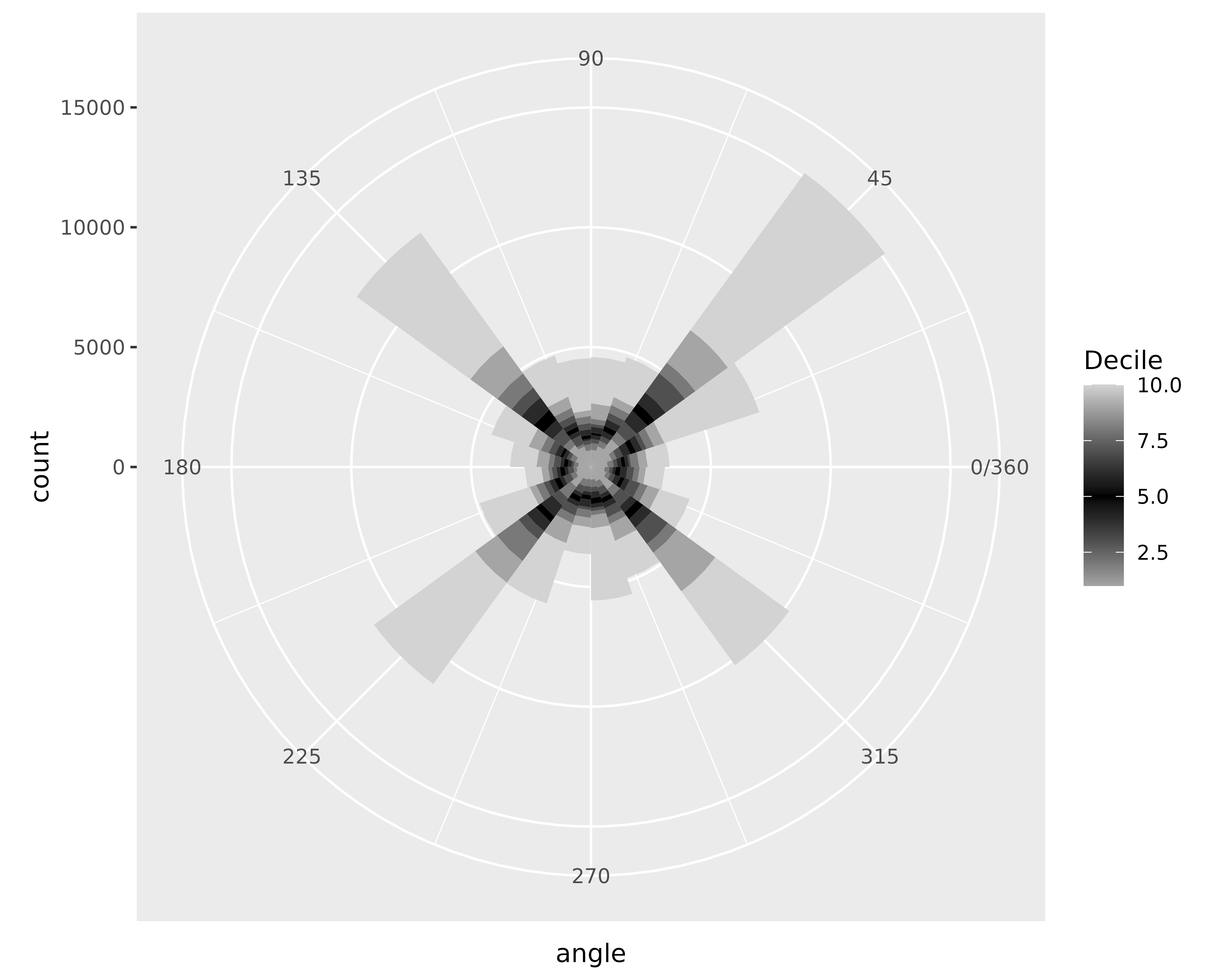
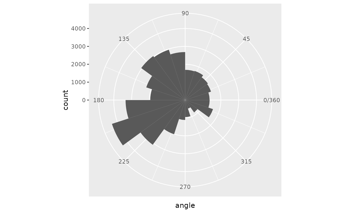
100 Attempts

In the end, the graph displays prominent trends in the diagonals. There are at least two reasons for this to appear (but I suspect there might be more).

1. The possible movement values range from around -1 to 1 for each direction before standardizing. This sets up a square of possible combinations. There are more combinations along the diagonals than in the cardinal directions. So, diagonals appear more often.
2. There are strange correlations between the simplex noise values. The hills and valleys between the two terrains sometimes match up on top of each other. These situations (or anywhere the difference in absolute value is very close) hit along a diagonal.

I like the strong tendency for diagonal movement, but there are options if you do not want that in your code. First, you can add a random rotation constant (like what happens to hue when setting up the colors), which will spin the trend away from the diagonals. Using a weighting scheme for the x and y directions, possibly using another round of simplex noise, can break apart the correlations. Finally, different parameters for simplex noise or other noise-generating functions can have different properties.