Libraries
The tidyverse makes this package easy to use. The golden ratio sets up the correct proportions for several measurements. So, we’ll save it as a global variable for this vignette.
library(penrosetiling)
library(tidyverse)

g_ratio <- (1 + sqrt(5)) / 2
Background
This package uses Robinson triangles to subdivide the rhombi in Penrose tiling. These triangles have specific proportions, and the subdivision follows a set of rules. The first example displays the four types of triangles. Regardless of their position, the triangles’ types assume they’re sitting flat with the two equal sides pointing upwards. There are two shapes, “t” for thin and “T” for thick, and two directions, left and right. Left triangles have their first point on the left side of the middle point. Right triangles are flipped. For the functions in this package, data sets with triangles will need the following columns: triangle for triangle id, rhombus for rhombus id, point1_x, point1_y, point2_x, point2_y, point3_x, and point3_y for coordinates.
The following code creates an introduction data set with each of the four triangles. The pivot_down function drops the data set from one row per triangle to one row per point with a new point column.
tiles <- data.frame(triangle = seq(1, 4),
                    shape = c("t", "t", "T", "T"),
                    point1_x = c(0, 2.5, 3, 5.5 + 2),
                    point1_y = c(0, 0, 0, 0),
                    point2_x = c(g_ratio * cos(72 * pi/180),
                                 1.5 + g_ratio * cos(72 * pi/180),
                                 3 + 2 * (1/g_ratio) * cos(36 * pi/180),
                                 5.5 + 2 * (1/g_ratio) * cos(36 * pi/180)),
                    point2_y = c(g_ratio * sin(72 * pi/180),
                                 g_ratio * sin(72 * pi/180),
                                 2 * (1/g_ratio) * sin(36 * pi/180),
                                 2 * (1/g_ratio) * sin(36 * pi/180)),
                    point3_x = c(1, 1.5, 3 + 2, 5.5),
                    point3_y = c(0, 0, 0, 0),
                    rhombus = seq(1, 4))

tiles_start <- pivot_down(tiles) %>%
  group_by(triangle) %>%
  mutate(mean_x = mean(x),
         mean_y = mean(y)) %>%
  mutate(label_x = .66 * x + .34 * mean_x,
         label_y = .66 * y + .34 * mean_y)

ggplot(tiles_start) +
  geom_polygon(aes(x = x,
                   y = y,
                   fill = shape,
                   group = triangle)) +
  geom_text(aes(x = label_x,
                y = label_y,
                label = point)) +
  scale_fill_manual(values = c("#FFC749",
                               "#B0E2FF")) +
  coord_equal() +
  theme_void() +
  theme(legend.position = "bottom")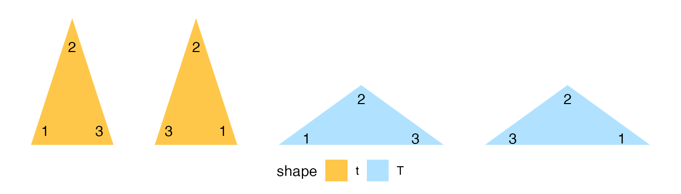
The output shows the four triangles with each of their points labels. For example, the left triangles have corner 1 to the left of the corner pointing upwards. If these triangles were rotated upside down, points 1 and 3 would not flip sides, and the triangles’ direction would stay the same. Therefore, left triangles always have point 1 to the left of point 2 when viewing the triangle from the edge connecting points 1 and 3.
substitution Function
The substitution function subdivides each triangle appropriately, depending on shape and direction. It will return a larger data set of smaller triangles. The smaller triangles have specific shapes and directions based on the input triangles.
tiles_substitution <- substitution(tiles)

tiles_substitution <- pivot_down(tiles_substitution) %>%
  group_by(triangle) %>%
  mutate(mean_x = mean(x),
         mean_y = mean(y)) %>%
  mutate(label_x = .66 * x + .34 * mean_x,
         label_y = .66 * y + .34 * mean_y)

ggplot(tiles_substitution) +
  geom_polygon(aes(x = x,
                   y = y,
                   fill = shape,
                   group = triangle)) +
  geom_text(aes(x = label_x,
                y = label_y,
                label = point)) +
  scale_fill_manual(values = c("#FFC749",
                               "#B0E2FF")) +
  coord_equal() +
  theme_void() +
  theme(legend.position = "bottom")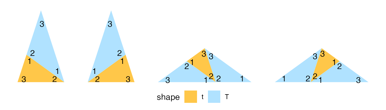
The first triangle was thin and left. The substitution function subdivided it into two smaller left triangles, one thin and one thick. The thick triangles convert into three smaller ones.
Starting Data Sets
Two functions provide data sets to start coding.
The return_rhombus function takes a starting position and shape to create a data set with two observations: two triangles that make up a rhombus.
tiles_1 <- return_rhombus(0, 0, -90 + 36, 2, 'T') %>%
  pivot_down() %>%
  group_by(triangle) %>%
  mutate(level = 1)

tiles_2 <- return_rhombus(0, 0, -90 + 36, 2, 'T') %>%
  substitution() %>%
  pivot_down() %>%
  group_by(triangle) %>%
  mutate(level = 2)

tiles_5 <- return_rhombus(0, 0, -90 + 36, 2, 'T') %>%
  substitution() %>%
  substitution() %>%
  substitution() %>%
  substitution() %>%
  substitution() %>%
  pivot_down() %>%
  mutate(level = 5)

tiles <- bind_rows(tiles_1, tiles_2, tiles_5)

ggplot(tiles) +
  geom_polygon(aes(x = x,
                   y = y,
                   fill = shape,
                   group = triangle)) +
  coord_equal() +
  facet_wrap(~ level)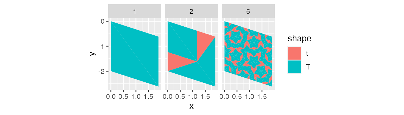
tiles_1 <- return_rhombus(0, 0, 0, 1 / sin(72 * pi/180), 't') %>%
  pivot_down() %>%
  group_by(triangle) %>%
  mutate(level = 1)

tiles_2 <- return_rhombus(0, 0, 0, 1 / sin(72 * pi/180), 't') %>%
  substitution() %>%
  pivot_down() %>%
  group_by(triangle) %>%
  mutate(level = 2)

tiles_5 <- return_rhombus(0, 0, 0, 1 / sin(72 * pi/180), 't') %>%
  substitution() %>%
  substitution() %>%
  substitution() %>%
  substitution() %>%
  substitution() %>%
  pivot_down() %>%
  mutate(level = 5)

tiles <- bind_rows(tiles_1, tiles_2, tiles_5)

ggplot(tiles) +
  geom_polygon(aes(x = x,
                   y = y,
                   fill = shape,
                   group = triangle)) +
  coord_equal() +
  facet_wrap(~ level)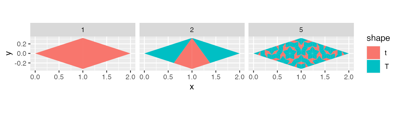
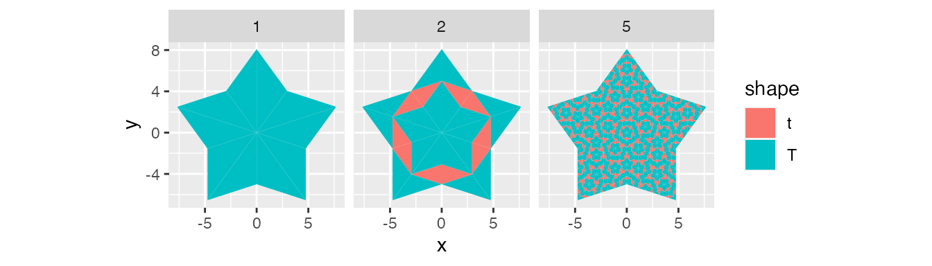
The return_starting_circle function also takes a starting position and shape to create a data set. This time the data set has ten observations. Either five rhombi or ten half rhombi, depending on the type of triangle.
tiles_1 <- return_starting_circle(0, 0, 0, 10, 't') %>%
  pivot_down() %>%
  mutate(level = 1)

tiles_2 <- return_starting_circle(0, 0, 0, 10, 't') %>%
  substitution() %>%
  pivot_down() %>%
  mutate(level = 2)

tiles_5 <- return_starting_circle(0, 0, 0, 10, 't') %>%
  substitution() %>%
  substitution() %>%
  substitution() %>%
  substitution() %>%
  substitution() %>%
  pivot_down() %>%
  mutate(level = 5)

tiles <- bind_rows(tiles_1, tiles_2, tiles_5)

ggplot(tiles) +
  geom_polygon(aes(x = x,
                   y = y,
                   fill = shape,
                   group = triangle)) +
  coord_equal() +
  facet_wrap(~ level)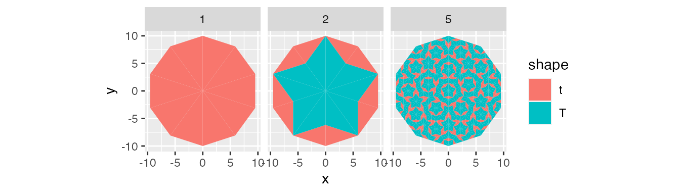
tiles_1 <- return_starting_circle(0, 0, 90, 5, 'T') %>%
  pivot_down() %>%
  mutate(level = 1)

tiles_2 <- return_starting_circle(0, 0, 90, 5, 'T') %>%
  substitution() %>%
  pivot_down() %>%
  mutate(level = 2)

tiles_5 <- return_starting_circle(0, 0, 90, 5, 'T') %>%
  substitution() %>%
  substitution() %>%
  substitution() %>%
  substitution() %>%
  substitution() %>%
  pivot_down() %>%
  mutate(level = 5)

tiles <- bind_rows(tiles_1, tiles_2, tiles_5)

ggplot(tiles) +
  geom_polygon(aes(x = x,
                   y = y,
                   fill = shape,
                   group = triangle)) +
  coord_equal() +
  facet_wrap(~ level)